Note 12/2012: Well, John Cole and I chatted by e-mail regarding the FMS 2 alpha 8 POLAR and he came up with a great way to create your own if you know the typical POLAR data for another airfoil. Below is what John sent to me. I hope you enjoy the details and his spreadsheet for making your own POLAR data for FMS and other RC sims.

As we've said before, Mr. Masuoka's .par editor is invaluable for making a correct FMS alpha8 .par file and serves as a better explanation in how the .par file is configured.

Get ParEdit.exe here: http://sekiai.net/fms_e.html#A8Editor_Converter
or in japanese at: http://www.ac.cyberhome.ne.jp/~v-tails/delphi/index.html.

---

* * * * John Cole Introduction * * * *

I felt that the .par files used for some FMS 8 planes could be made a bit more realistic. Compared with my real models (which are all easy-fly types, both electric and i/c) the FMS models seemed to glide rather steeply power-off, and did not seem to stall correctly. I decided I would modify various parts of one to get it to “fly better”.

I based my work on an old FMS 7 model: the SuperCup, and used the 7 to 8 par converter written by Masuoka Hideaki, and then edited the resulting .par file using his ParEdit program – as well as just using a text editor. It’s generally easier to use ParEdit as you can see more easily what you’re changing, and usually there’s a label which tells you whether you want positive or negative change. Some changes can be seen “visually” in the 3-D view. What follows assumes that’s how you’re doing your edit, except where I explain that I used a text-editor.

* * * * What’s in the .par file? * * * *

A lot. For me the most important bits were the parts that determine how the plane flies. These are the amount of power, the weight, the moments of inertia (which determine the force needed to rotate the plane in each of the 3 axes: roll, pitch and yaw), the size and location of the “flying surfaces”, and the aerodynamic coefficients of each of those surfaces. The surfaces are the two wings (left and right, or 4 for a biplane), the stabiliser / elevator, the rudder / fin and the fuselage. Each is described by its dimensions and location relative to the model centre, and its aerodynamic coefficients – the polar.

Note that the fuselage is described in a special way: as two items: a long thin “plank” with length and height (but no thickness) which gives lift (and drag) when the model is yawing (e.g. in knife-edge flight), and a drag-only component which reflect the profile drag of everything except the main flying surfaces – so including the undercarriage. The aerodynamic forces on e.g. the left wing are calculated separately for several elements. Typically 4 or 5, with each element being a part of the span. This means that in a turn, the calculation of lift and drag for e.g. the wingtip will be separate from that near the root.

I made a few changes on the basis of “feel” and some simple calculations, and altered the Moments of Inertia so that the Yaw moment was about the same as the sum of the Roll and Pitch moments; that seemed to improve the responsiveness. I reduced the power (this is a Combustion model; reduce power by reducing max. fuel flow). I also reduced the Propeller Moment of Inertia, so the motor picked up quicker.

* * * * The Polars * * * *

The main changes I made were to the parts of the .par file that are perhaps the most difficult to understand: the aerofoil polars. The SuperCup has 4 polars: wing, stabiliser, fin and fuselage. I altered the first 3, but the main change I made was to the wing polar (polar 1). I’ll describe here how I constructed the wing polar, as the same principle applies to the others – except that they are simpler to build as they represent symmetric sections.

Once I had changed the wing polar, I had to make a couple of other: I moved the centre of gravity with respect to the wing chord (do this by moving the wing position forward), and I also increased the wing incidence. Easy with ParEdit. The tricky bit was redesigning the polars. Let me explain how they are put together.

The .par files are simple text files containing all the rules about how a specific plane flies. As well as this data, there are comments for you to read but which FMS ignores. Comments start with // and all text on a line following (and including) the // is ignored by FMS. Each wing (also stabiliser etc.) is described by its dimensions and position and marked with a number of its polar; each wing (right and left) is described differently.

For me, both of those wings used Polar 1. The description of the data in the polar tables, and the data I used, are shown towards the end of these notes, but they are mainly the three coefficients (Cl, Cd, Cm) of Lift, Drag and Pitching Moment for a full range of values of alpha (aerodynamic angle of attack). These coefficients are explained at the end of this note.

* * * * Sources of data for the Polars * * * *

Before I explain a bit about the data sources, let me make a comment on the wide range required: if you look in a text-book on aerodynamics, you’ll find that data is only given for the “normal” range – usually between the positive and negative stalling angles. But FMS needs a complete range through 360 degrees.

So where to get it? I found some data for vertical-axis wind turbines, which covers the full range. It’s referred to in a page called “Airfoils at High Angle of Attack”, at http://www.aerospaceweb.org/question/airfoils/q0150b.shtml but to get the full data including values for Cm, click this link at Sandia.gov and download the paper “Aerodynamic Characteristics of Seven Symmetrical Airfoil Sections Through 180-Degree Angle of Attack For Use In Aerodynamic Analysis of Vertical Axis Wind Turbines”.

The aerospaceweb page makes the useful point that, beyond the stall, the characteristics of all aerofoil sections are similar – even flat plates. So you can safely use data for one of their sections for the beyond-stall alpha, and data for your own section for the all-important “normal range” between positive and negative stall.

OK, so you have the wide-range data, but what about getting the normal-range data. You can get it from any aerodynamics source, but you will need it for the specific aerofoil section you want to use on your plane. I got my data from Model Aircraft Aerodynamic, by Martin Simons – (ISBN 1854861905).

For my model, I decided to use the Eppler 374 aerofoil – “semi-symmetric” with 2.25% camber and 10.9% thickness. That book (and any other similar source) contains wind-tunnel data on the three coefficients for each value of alpha, just as the above Sandia paper does. So you read these off the wind-tunnel charts and put them into a table (preferably a spreadsheet, as you’re going to do some sums on the values).

There are two points to note. The data you want are Cl, Cd and Cm. Sometimes there is a graph of Cl, Cd and Cm against alpha (sometimes on two sheets), and sometimes there’s a graph of Cl against alpha plus graphs of Cd and Cm against Cl. But either way you can read off Cl for a range of values of alpha, and then read Cd and Cm using either alpha or Cl as your “index”.

* * * * Don't Forget Mr. Reynolds * * * *

But when you look at the graphs in the book, there is more than one line? That’s because how well a section works depends on how fast it’s travelling. The way this is reflected is to use a special unit-less number which reflects this speed (the Reynolds Number – Re), and so each line in the text-book’s graph applies to one value of Re. If you set the display correctly, FMS tells you how fast the model is flying. For me this varies between 7 and 28 metres / second (usually 14 – 21). You calculate Re as follows if you are working in metric units: multiply speed (m/s), wing chord (m) and 68459. So 14 m/s and a wing chord of 0.36 metres gives Re of about 345,000. My book’s data include a line for Re of 250,000 for E374 and that’s what I used. Small, light (Indoor) planes fly at much lower Re, and you will need to use a different line for them.

* * * * Correcting for In-wash / Out-wash and Vortex-induced drag * * * *

So now you combine the two sources of data. I used the model book data for alpha of -15 to +15 degrees, and the turbine data for the rest of the full range. But these data are (effectively) for an endless wing. You need to do two things, both quite straightforward, to reflect the aspect ratio (about 5 in my case): Correct the data for inwash / outwash as alpha increases, and add to the drag coefficient Cd the vortex-induced drag Cdi.

As alpha increases, the air pressure under the wing increases and that over the wing decreases. At the wingtip, air tends to slide in towards the root on the upper surface and out towards the tip on the under-surface. The effect of this is to reduce the local alpha. It’s like walking up a steep hill: if you walk diagonally, your path is less steep that the line straight up the hill. For many sections, Cl increases at 0.11 per degree alpha for an endless wing. Reducing this to about 0.09 per degree alpha is a rough correction for this effect.

So I took as my basis the zero-lift alpha (-2 degrees for E374) and INCREASED the tabulated values of alpha (in the normal range) by adding 20% to their (value + 2). So I converted 6 degrees (plus 2 = 8 degrees above the zero-lift angle) to 9.6 degrees (above zero lift: 8 * 1.2), or 7.6 degrees “true” (9.6 – 2). So my table entry for 6 degrees alpha was changed to 7.6 degrees alpha. I did this for the “normal range” but did not bother outside that. So now, you need to increase the wing incidence to reflect this. My table entry for (old) 6 degrees showed a Cl of 0.6 – about right for a slow cruise. So to achieve that Cl in practice you need a corrected alpha of 7.6 degrees. So I increased the incidence by 2 degrees (a bit more than I needed to).

Also, as alpha increases, the wingtip vortex becomes stronger – and that creates induced / vortex drag. Its coefficient Cdi is calculated as K times (CL squared), divided by (Pi times A) where A is the aspect ratio. K is a constant that varies with the wing planform, but take K = 1 and you’ll be reasonably close. So for each value of corrected alpha, add to Cd an amount calculated using that formula. This extra drag is just 10% at corrected alpha of 0.4 degrees (2.4 degrees above the zero-lift angle of -2 degrees for E374), but doubles the drag at alpha = 7.6 degrees.

So, now you have a table with Cl, Cd (inc Cdi) and Cm for a range of (corrected) alpha values. All you do is put these values (4 to a line: alpha, Cl, Cd, Cm as decimal numbers separated by a single space) as the first part of your Polar 1, prefixed by a number saying how many data points there are (i.e. how many values of alpha). This is the one time it’s easier to use a text editor: just copy and paste!

OK, now you know how to do it, get your spreadsheet ready and calculate your OWN .par file!

* * * * The data from my .par file for Polar 1 * * * *

The Polar data (for each polar) is in two parts: first, a list of how the aerofoil behaves at a large number of angles of attack (alpha) – this section is prefixed by a number saying how many points there are. The second section contains just three numbers, which all relate to “flow separation”. Let me be a bit simplistic and say that means the same as stalling. The three numbers set out the (negative) angle at which the wing stalls nose-down, the (positive) angle at which it stall nose-up, and the hysteresis angle. The last of these is the difference between the angle at which a wing stalls, and the angle you have to bring it back to for it to unstall. So e.g. if a wing stalls at an alpha of 15 degrees but won’t unstall until you bring that down to 13 degrees then the hysteresis is 2 degrees.

The aerofoil performance data comprises three numbers for each value of alpha: Cl (the lift coefficient) Cd (the drag coefficient) and Cm (the Moment coefficient). These data need to be given for the full range of alpha (-180 degrees through zero through to +180 degrees – note that here both + and – 180 degrees refer to the wing flying backwards!). Typically, polars contain between 15 and 40 datapoints; my polar 1 uses 26.

Just a brief comment on what these are: first, they are all “coefficients” – unit-less numbers that are the same whether you work in metres or feet. As you would guess, Cl tells you how effective the section is at creating Lift, and Cd Drag. It’s a convention that in a wind-tunnel these two forces are measured at right-angles to the direction of flow, and parallel to it. They are NOT measured relative to the section’s axis – that obviously changes direction as the wing section is tilted to vary alpha.

But what’s Cm? In the old days it was discovered that changing alpha altered not only the lift but where that lift seemed to act. Increasing alpha brought the “centre of lift” forward, and reducing it sent it back. Then it was realized that this could be more conveniently be described by always measuring the lift force at the 25% point of the wing chord, and simultaneously measuring the pitching moment measured about this 25% point.

This pitching moment in the normal range is nose-down for a cambered-section, and there is no pitching moment for a symmetric section. For many cambered wing sections (including E 374), Cm is essentially constant and negative (nose-down) in the “normal range”. Note that once you pass the stall the Cm for both cambered-section and symmetric section aerofoils is large and negative (nose down) for a positive-alpha stall. Note: a “cambered” section is one where the “mean line” (i.e. the centre line) of the section is cambered (or curved). Flat-bottomed sections like Clark Y are in fact cambered sections.

//POLAR1
26                       //Number of points
-180.00 0.00 0.00 0.00   //Alpha (deg), CL, CD, CM
-170.00 0.81 0.17 0.00
-160.00 0.58 0.33 0.05
-150.00 0.70 0.63 0.10
-140.00 0.90 0.99 0.15
-90.00 -0.07 1.84 0.50
-45.00 -0.96 1.13 0.25
-10.00 -0.50 0.14 0.10
-8.00 -0.60 0.12 0.04
-6.00 -0.50 0.09 -0.03
-2.00 0.00 0.030 -0.07
0.40 0.20 0.022 -0.07
7.60 0.60 0.039 -.07
12.40 0.90 0.063 -0.07
14.80 0.85 0.098 -0.07
17.20 0.80 0.134 -0.20
20.80 0.58 0.234 -0.20
23.00 0.58 0.36 -0.20
33.00 0.88 0.74 -0.20
45.00 0.96 1.13 -0.25
90.00 0.07 1.84 -0.50
140.00 -0.90 0.99 -0.15
150.00 -0.70 0.63 -0.10
160.00 -0.58 0.33 -0.05
170.00 -0.81 0.17 0.00
180.00 0.00 0.00 0.00
-7                         //angle of attack lower flow separation [deg]
15                         //angle of attack upper flow separation [deg]
1                          //flow separation hysteresis [deg]

* * * * Looking at the Polar 1 data using ParEdit * * * *

If you open your .par file with ParEdit and select the Wing and Polar 1, and then click the Polar View tab on the right side you’ll see a graph. There are two possible views, selected on the tab just below Polar.

Here’s my data Polar viewed that way:

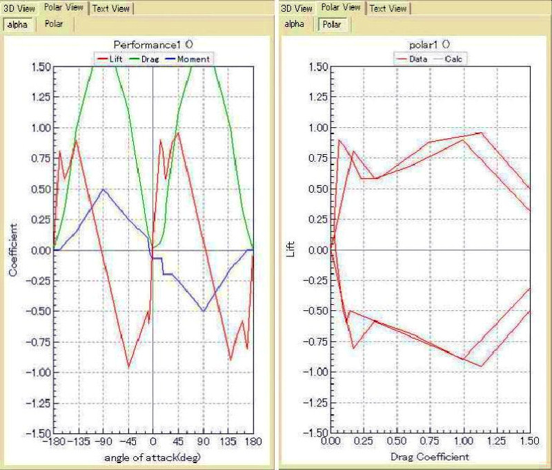
If you look at the left-hand (Alpha) graph you’ll see that as alpha rises from zero, the red (Cl) values rise, peak, fall, then more slowly rise again to a second peak. The first peak is the beginning of the (nose-up) stall. With E374 the nose-down stall is less pronounced. At the nose-up stall, Cm (blue) suddenly changes from slightly-negative to strongly-negative. That’s characteristic of positive-camber sections like E374. Cd (green) is small near alpha = zero, increasing very steeply as you pass the stall.

The second graph plots Cl (vertical) against Cd (horizontal), and again shows low Cd for alpha near zero. This type of plot is sometimes called a polar-plot.

If you compare the graphs here with those of other .par files you will see that Cl rises here to a peak at about 12 degrees alpha, and the subsequent fall of 33% is larger than in some other .par files – emphasising the stall. I have not spotted another .par file that seems to include either inflow / outflow correction or induced drag correction.

Note 12/2012: I asked John to provide a bit more detail regarding how to use the spreadsheet to create the .par file text to paste into the FMS 2 alpha8 .par file. Here's a link to his response with more details for saving the spreadsheet data to the .par file.

THE END